The Graph of an Analysis — ggfacto • ggfacto

The graph of a multiple correspondence analysis, a correspondence analysis or a principal component analysis, in the plane of two axes — one verb for the three, as interpret is their one table:

a multiple correspondence analysis draws its active levels, and behind them the cloud of its individuals as answer profiles (see ggmca);
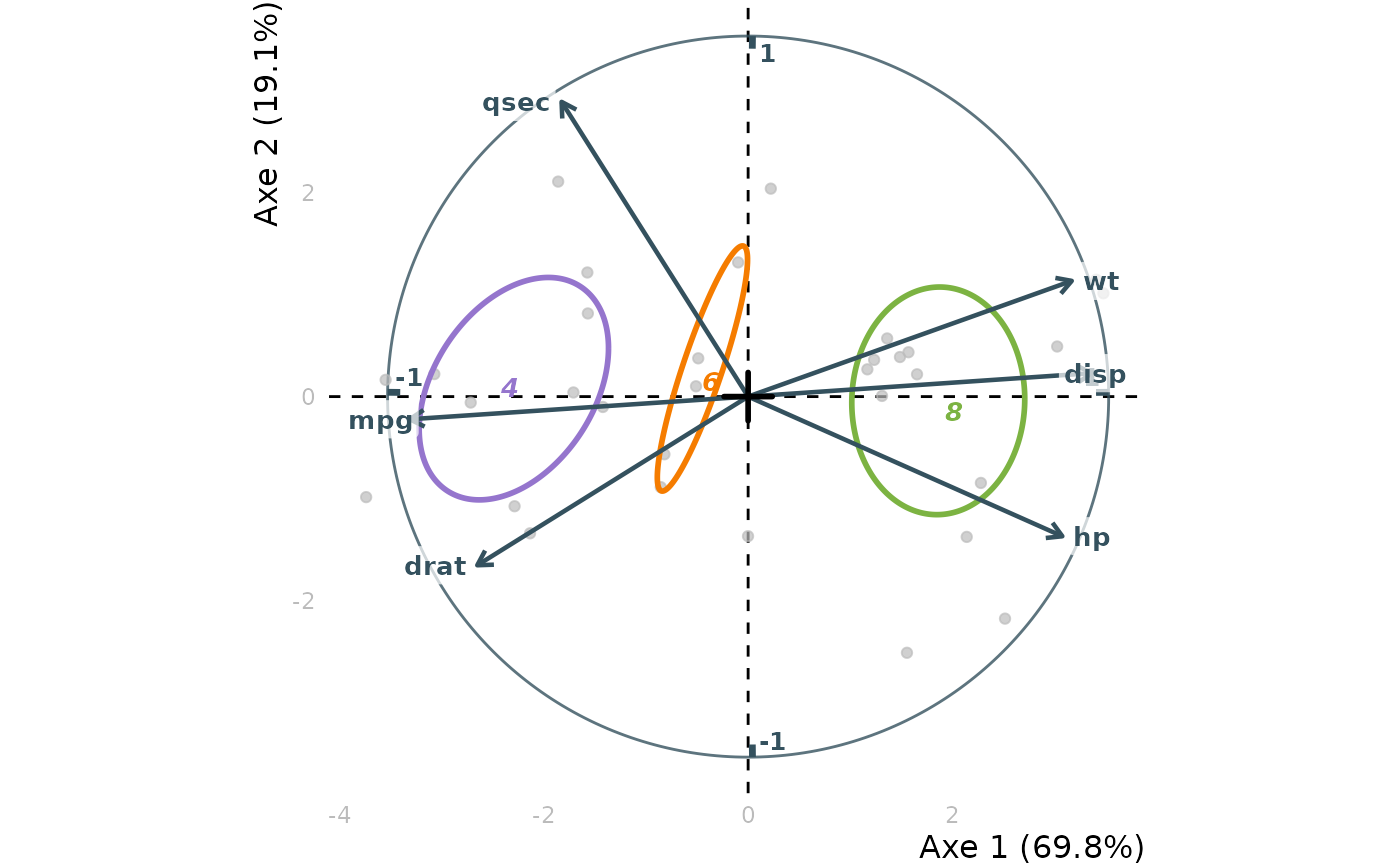
a correspondence analysis draws the levels of its two variables, and of the supplementary variables its table holds (see ggca);
a principal component analysis draws its biplot: the cloud of the individuals with the variables' arrows rescaled onto it (see ggpca); `profiles = FALSE` draws its circle of correlations (see ggpca_cor_circle).

Hovering a point shows the data behind it: a level's crosstabs, coloured by their deviations from the mean, an individual's answers or values, a supplementary level's percentages or means. Supplementary variables and clusters are added from the data frame, for an MCA or a PCA, and from the table, for a CA.

Usage

ggfacto(
  res,
  data,
  sup_vars,
  clust,
  axes = c(1, 2),
  axes_reverse = NULL,
  type,
  profiles = TRUE,
  active_tables,
  ellipses = NULL,
  title,
  xlim,
  ylim,
  text_size = 3.5,
  size_scale_max = NULL,
  lang = NULL,
  interactive = FALSE,
  ...
)

Arguments

res: An analysis made with multiple_correspondence_analysis, correspondence_analysis or principal_component_analysis (or with FactoMineR::MCA(), CA() or PCA(), or GDAtools::speMCA() or csMCA()).
data: The data frame the analysis was made on, in which to find the supplementary variables and the clusters, for an MCA or a PCA: the whole data frame, even when the analysis was made on a subset of it. A CA reads its table instead.
sup_vars: <tidy-select> The supplementary variables, as in `tab()`: `sup_vars = c(SEX, AGE)`. For a CA, they are the table's other variables: `tab(data, c(relig, marital), c(partyid, race))`.
clust: The clusters, made with hierarchical_clust: for an MCA or a PCA, the column of `data` that holds them (`clust = cah`); for a CA, the clusters of the levels of one margin (`clust = hierarchical_clust(res, ncp = 2, nb_clust = 4)`).
axes: The axes to draw, as a numeric vector of length 2.
axes_reverse: `1` to invert left and right, `2` to invert up and down, `1:2` for both.
type: How the levels are drawn: "text", "labels" or "points", and "facets" for one graph per level of the first supplementary variable (MCA, PCA). By default "text", and "points" for a CA.
profiles: Should the cloud of the individuals be drawn? As answer profiles for an MCA, as a biplot for a PCA. By default, yes; `FALSE` draws the levels alone, and a PCA's circle of correlations when nothing else is asked for.
active_tables: The crosstabs in the tooltips of an MCA: see ggmca.
ellipses: A number between 0 and 1 draws a concentration ellipse around the individuals of each level of the first supplementary variable: 0.5 holds half of them.
title: The title of the graph.
xlim, ylim: Horizontal and vertical limits, as numeric vectors of length 2.
text_size: Size of text.
size_scale_max: The size of the largest point. By default, computed from the spread of the weights of the points drawn.
lang: NULL (the session's language), "en" or "fr": the language of the tooltips and of the axis titles.
interactive: Set to TRUE to get the interactive graph at once, as ggi makes it. By default, a ggplot2 graph, to which elements can be added with `+`, before passing it to ggi.
...: Further arguments of the analysis's own graph function, which document them: ggmca (such as `tooltip_vars`, `max_profiles`, `color_groups`), ggca (`show_sup`, `uppercase`, `tooltips`) or ggpca.

Value

A ggplot object, or an html widget with `interactive = TRUE`.

Details

An argument that an analysis does not take stops with an explanation: `data`, `sup_vars`, `profiles`, `active_tables` and `ellipses` for a CA, `active_tables` for a PCA.

Examples

# \donttest{
data(tea, package = "FactoMineR")
res.mca <- multiple_correspondence_analysis(tea, 1:18)
tea <- tea |>
  dplyr::mutate(clust = hierarchical_clust(res.mca, ncp = 3, nb_clust = 5))
ggfacto(res.mca, tea, sup_vars = SPC, clust = clust, interactive = TRUE)


gss <- forcats::gss_cat |>
  dplyr::filter(!relig %in% c("No answer", "Don't know", "Not applicable"),
                !partyid %in% c("No answer", "Don't know"))
res.ca <- correspondence_analysis(tabxplor::tab(gss, c(relig, marital), partyid))
ggfacto(res.ca, interactive = TRUE)


cars <- mtcars
cars$cyl <- factor(cars$cyl)
res.pca <- principal_component_analysis(cars, c(mpg, disp, hp, drat, wt, qsec))
ggfacto(res.pca, cars, sup_vars = cyl, ellipses = 0.5)
#> Warning: Probable convergence failure

# }