Plot Initial Dimensions (Active Variables) on a Multiple Correspondence Analyses
Source:R/mca-teach.R
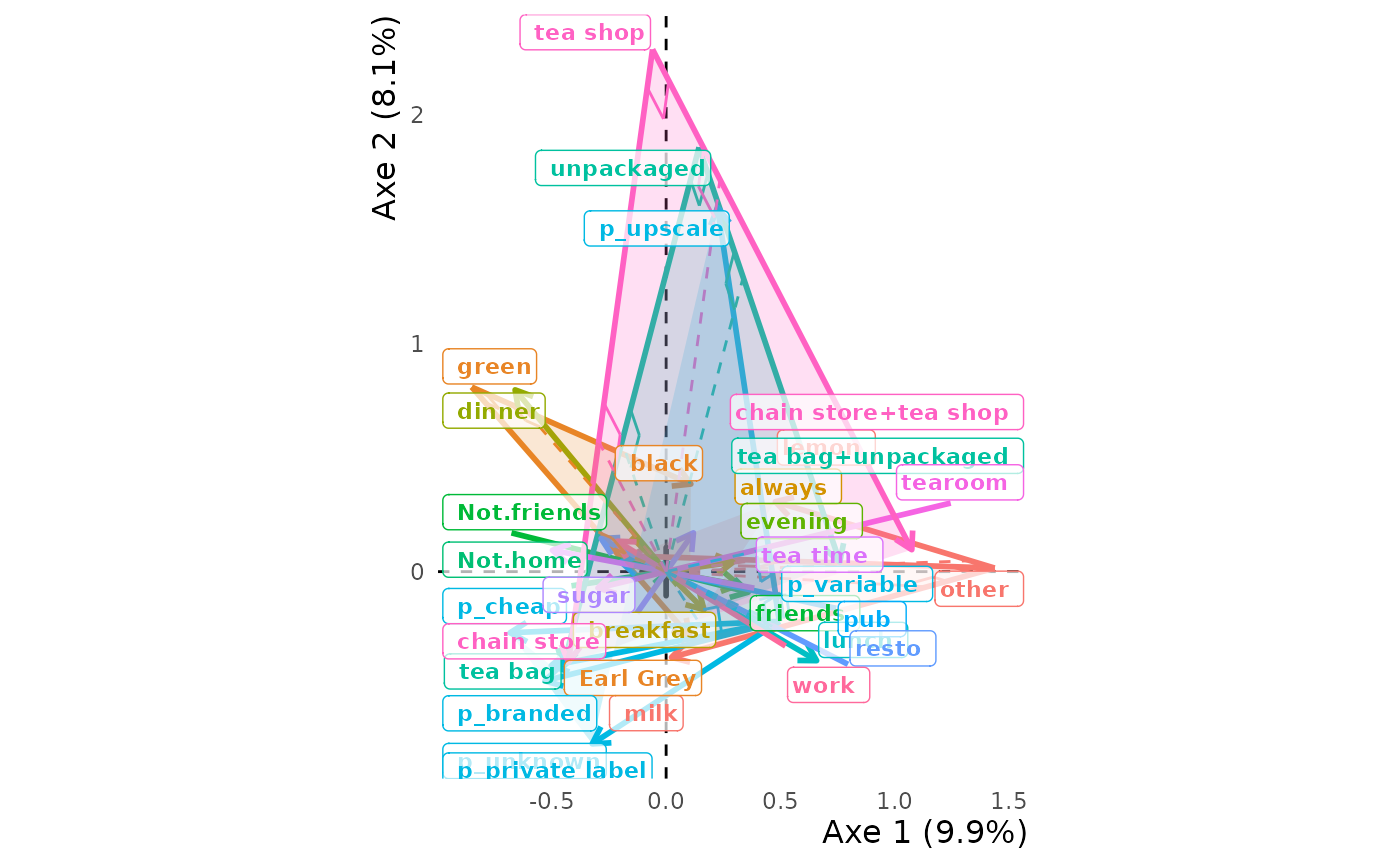
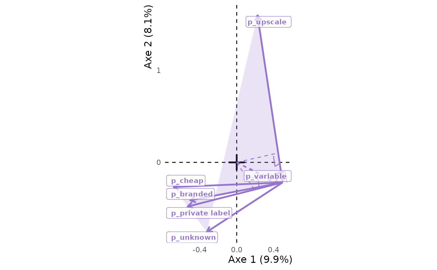
ggmca_with_base_ref.RdThis function mostly have an educational value : it shows the
initial dimensions of the Multiple Correspondence Analysis (active variables)
in the space built by the analysis (principal axes). To see initial
dimensions in their initial reference frame, use ggmca_initial_dims.
Usage
ggmca_with_base_ref(res.mca, data, axes = c(1, 2), keep = NULL)Arguments
- res.mca
An object created with
FactoMineR::MCA.- data
The data the analysis was made on. Optional: this graph draws only active variables, which are read from `res.mca`, so it changes nothing. It is accepted so that every `ggmca_*` function takes `(res.mca, data)`.
- axes
The axes to print, as a numeric vector of length 2.
- keep
A character vector of the name of active variables to keep.
Value
A ggplot object to be printed in the
`RStudio` Plots pane. Possibility to add other gg objects with +.
Sending the result through ggi will draw the
interactive graph in the Viewer pane using girafe.
Examples
# \donttest{
data(tea, package = "FactoMineR")
res.mca <- multiple_correspondence_analysis(tea, 1:18)
ggmca_with_base_ref(res.mca)
#> Warning: Removed 18 rows containing missing values or values outside the scale range
#> (`geom_segment()`).
#> Warning: Removed 18 rows containing missing values or values outside the scale range
#> (`geom_segment()`).
#> Warning: Removed 13 rows containing missing values or values outside the scale range
#> (`geom_segment()`).
#> Warning: Removed 31 rows containing missing values or values outside the scale range
#> (`geom_segment()`).
#> Warning: Removed 31 rows containing missing values or values outside the scale range
#> (`geom_segment()`).
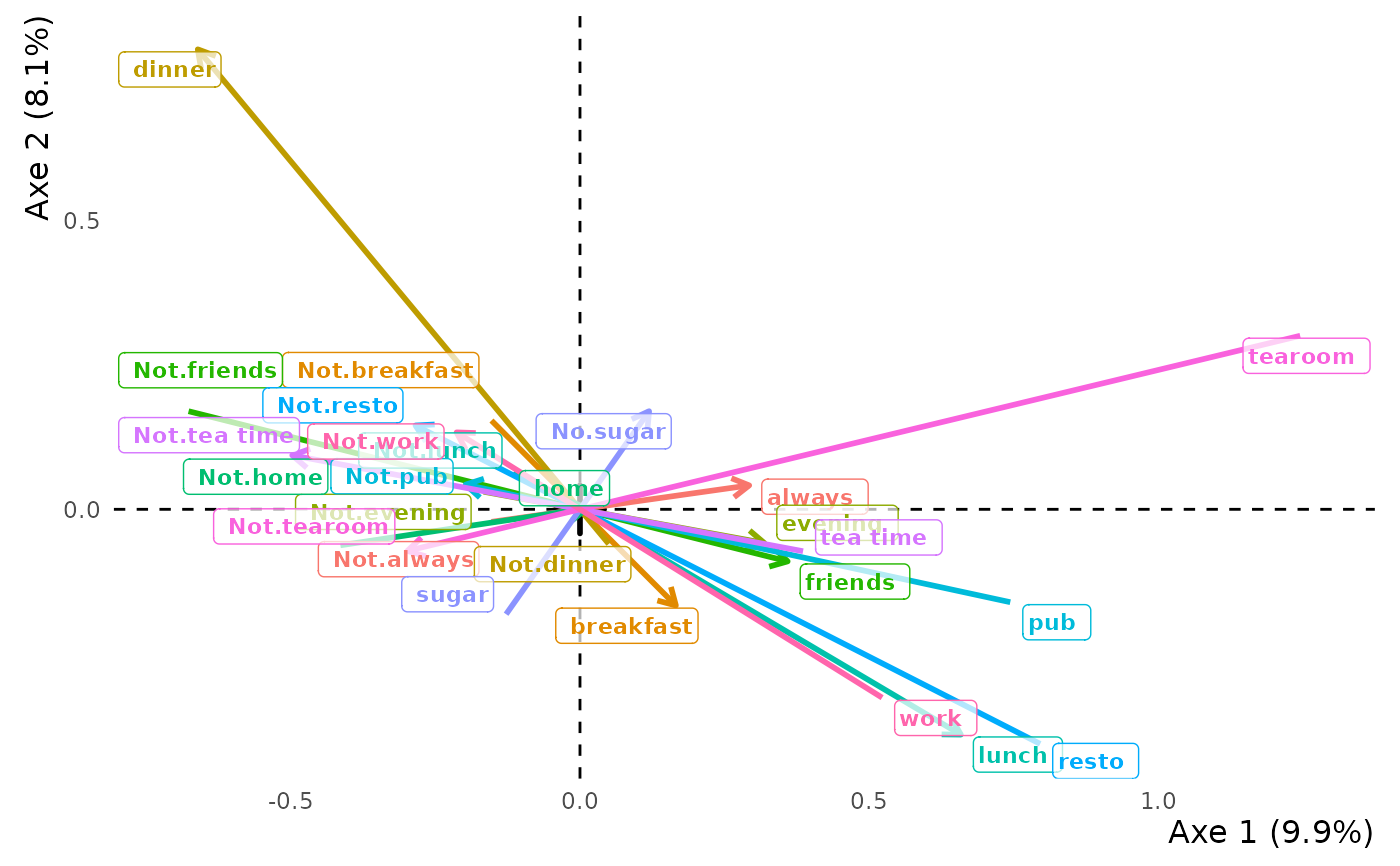
 # It is more readable to select just a few active variables
lv2_vars <- dplyr::select(tea[1:18], where(~ nlevels(.) == 2)) |> names()
ggmca_with_base_ref(res.mca, keep = lv2_vars)
#> Warning: Removed 13 rows containing missing values or values outside the scale range
#> (`geom_segment()`).
#> Warning: Removed 13 rows containing missing values or values outside the scale range
#> (`geom_segment()`).
#> Warning: Removed 13 rows containing missing values or values outside the scale range
#> (`geom_segment()`).
#> Warning: Removed 26 rows containing missing values or values outside the scale range
#> (`geom_segment()`).
#> Warning: Removed 26 rows containing missing values or values outside the scale range
#> (`geom_segment()`).
# It is more readable to select just a few active variables
lv2_vars <- dplyr::select(tea[1:18], where(~ nlevels(.) == 2)) |> names()
ggmca_with_base_ref(res.mca, keep = lv2_vars)
#> Warning: Removed 13 rows containing missing values or values outside the scale range
#> (`geom_segment()`).
#> Warning: Removed 13 rows containing missing values or values outside the scale range
#> (`geom_segment()`).
#> Warning: Removed 13 rows containing missing values or values outside the scale range
#> (`geom_segment()`).
#> Warning: Removed 26 rows containing missing values or values outside the scale range
#> (`geom_segment()`).
#> Warning: Removed 26 rows containing missing values or values outside the scale range
#> (`geom_segment()`).
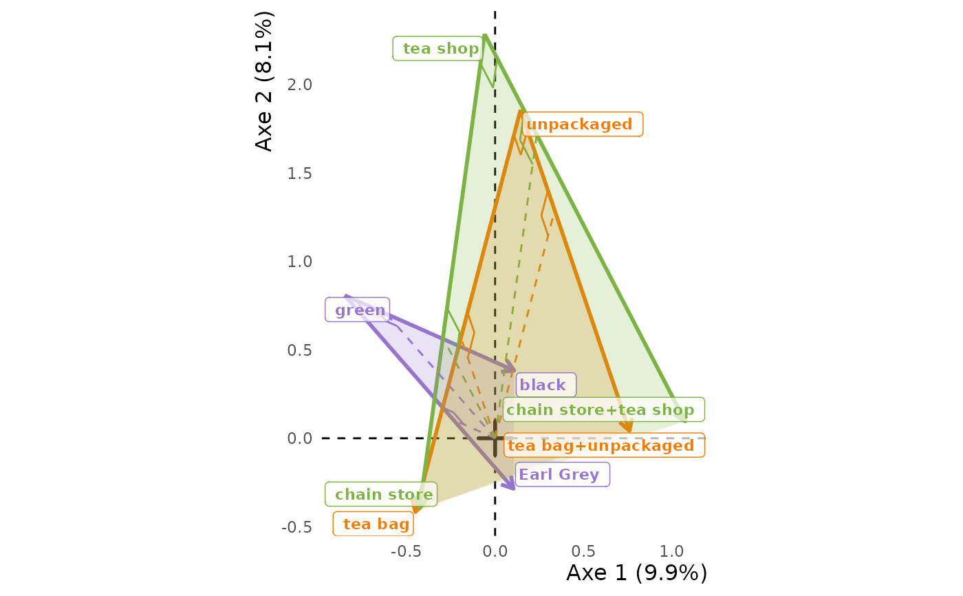
 lv3_vars <- dplyr::select(tea[1:18], where(~ nlevels(.) == 3)) |> names()
ggmca_with_base_ref(res.mca, keep = lv3_vars)
#> Warning: Removed 3 rows containing missing values or values outside the scale range
#> (`geom_segment()`).
#> Warning: Removed 3 rows containing missing values or values outside the scale range
#> (`geom_segment()`).
#> Warning: Removed 3 rows containing missing values or values outside the scale range
#> (`geom_segment()`).
#> Warning: Removed 3 rows containing missing values or values outside the scale range
#> (`geom_segment()`).
lv3_vars <- dplyr::select(tea[1:18], where(~ nlevels(.) == 3)) |> names()
ggmca_with_base_ref(res.mca, keep = lv3_vars)
#> Warning: Removed 3 rows containing missing values or values outside the scale range
#> (`geom_segment()`).
#> Warning: Removed 3 rows containing missing values or values outside the scale range
#> (`geom_segment()`).
#> Warning: Removed 3 rows containing missing values or values outside the scale range
#> (`geom_segment()`).
#> Warning: Removed 3 rows containing missing values or values outside the scale range
#> (`geom_segment()`).
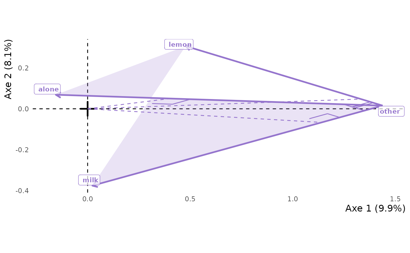
 lv4_vars <- dplyr::select(tea[1:18], where(~ nlevels(.) == 4)) |> names()
ggmca_with_base_ref(res.mca, keep = lv4_vars)
#> Warning: Removed 1 row containing missing values or values outside the scale range
#> (`geom_segment()`).
#> Warning: Removed 1 row containing missing values or values outside the scale range
#> (`geom_segment()`).
#> Warning: Removed 1 row containing missing values or values outside the scale range
#> (`geom_segment()`).
#> Warning: Removed 1 row containing missing values or values outside the scale range
#> (`geom_segment()`).
lv4_vars <- dplyr::select(tea[1:18], where(~ nlevels(.) == 4)) |> names()
ggmca_with_base_ref(res.mca, keep = lv4_vars)
#> Warning: Removed 1 row containing missing values or values outside the scale range
#> (`geom_segment()`).
#> Warning: Removed 1 row containing missing values or values outside the scale range
#> (`geom_segment()`).
#> Warning: Removed 1 row containing missing values or values outside the scale range
#> (`geom_segment()`).
#> Warning: Removed 1 row containing missing values or values outside the scale range
#> (`geom_segment()`).
 lv6_vars <- dplyr::select(tea[1:18], where(~ nlevels(.) == 6)) |> names()
ggmca_with_base_ref(res.mca, keep = lv6_vars)
#> Warning: Removed 1 row containing missing values or values outside the scale range
#> (`geom_segment()`).
#> Warning: Removed 1 row containing missing values or values outside the scale range
#> (`geom_segment()`).
#> Warning: Removed 1 row containing missing values or values outside the scale range
#> (`geom_segment()`).
#> Warning: Removed 1 row containing missing values or values outside the scale range
#> (`geom_segment()`).
lv6_vars <- dplyr::select(tea[1:18], where(~ nlevels(.) == 6)) |> names()
ggmca_with_base_ref(res.mca, keep = lv6_vars)
#> Warning: Removed 1 row containing missing values or values outside the scale range
#> (`geom_segment()`).
#> Warning: Removed 1 row containing missing values or values outside the scale range
#> (`geom_segment()`).
#> Warning: Removed 1 row containing missing values or values outside the scale range
#> (`geom_segment()`).
#> Warning: Removed 1 row containing missing values or values outside the scale range
#> (`geom_segment()`).
 # }
# }